Latent Dirichlet Allocation and Topic Modeling

When reading an article, we humans are able to easily identify the topics the article talks about. An interesting question is: can we automate this process, i.e., train a machine to find out the underlying topics in articles? In this post, a very popular topic modeling method, Latent Dirichlet allocation (LDA), will be discussed.

Latent Dirichlet Allocation (LDA) Topic Model¹

Given a library of \(M\) documents, \(\mathcal{L}=\{d_1,d_2,...,d_M\}\), where each document \(d_m\) contains a sequence of words, \(d_m=\{w_{m,1},w_{m,2},...,w_{m,N_m}\}\), we need to think of a model which describes how essentially these documents are generated. Considering \(K\) topics and a vocabulary \(V\), the LDA topic model assumes that the documents are generated by the following two steps:

• For each document \(d_m\), use a doc-to-topic model parameterized by \(\boldsymbol\vartheta_m\) to generate the topic for the \(n\)th word and denote it as \(z_{m,n}\), for all \(1 \leq n \leq N_m\);
• For each generated topic \(k=z_{m,n}\) corresponding to each word in each document, use a topic-to-word model parameterized by \(\boldsymbol\varphi_k\) to generate the word \(w_{m,n}\).

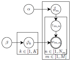
The two steps are graphically illustrated in Fig. 1. Considering that the doc-to-topic model and the topic-to-word model essentially follow multinomial distributions (counts of each topic in a document or each word in a topic), a good prior for their parameters, \(\boldsymbol\vartheta_m\) and \(\boldsymbol\varphi_k\), would be the conjugate prior of multinomial distribution, Dirichlet distribution.

A conjugate prior, \(p(\boldsymbol\varphi)\), of a likelihood, \(p(\textbf{x}|\boldsymbol\varphi)\), is a distribution that results in a posterior distribution, \(p(\boldsymbol\varphi|\textbf{x})\) with the same functional form as the prior (but different parameters). For example, the conjugate prior of a multinomial distribution is Dirichlet distribution. That is, for a multinomial distribution parameterized by \(\boldsymbol\varphi\), if the prior for \(\boldsymbol\varphi\) is a Dirichlet distribution characterized by \(Dir(\boldsymbol\varphi|\boldsymbol\alpha)\), after observing \(\textbf{x}\), the posterior for \(\boldsymbol\varphi\) still follows a Dirichlet distribution \(Dir(\boldsymbol\varphi|\textbf{n}_x+\boldsymbol\alpha)\), but incorporating the counting result \(\textbf{n}_x\) of observation \(\textbf{x}\).

Keep this in mind, let us take a closer look at the two steps:

1. In the first step, for the \(m\)th document, assume the prior for the doc-to-topic model's parameter \(\boldsymbol\vartheta_m\) follows \(Dir(\boldsymbol\vartheta_m|\boldsymbol\alpha)\), after observing topics in the document and obtaining the counting result \(\textbf{n}_m\), we have the posterior for \(\boldsymbol\vartheta_m\) as \(Dir(\boldsymbol\vartheta_m|\textbf{n}_m+\boldsymbol\alpha)\). After some calculation, we can obtain the topic distribution for the \(m\)th document as
   \begin{equation} p(\textbf{z}_m|\boldsymbol\alpha)=\frac{\Delta(\textbf{n}_m+\boldsymbol\alpha)}{\Delta(\boldsymbol\alpha)}, \end{equation}
   where \(\Delta(\boldsymbol\alpha)\) is the normalization factor for \(Dir(\textbf{p}|\boldsymbol\alpha)\), i.e., \(\Delta(\boldsymbol\alpha)=\int{\prod_{k=1}^K{p_k^{\alpha_k-1}}}d\textbf{p}\). Taking all documents into account,
   \begin{equation} \label{Eqn:Doc2Topic} p(\textbf{z}|\boldsymbol\alpha)=\prod_{m=1}^M{p(\textbf{z}_m|\boldsymbol\alpha)}=\prod_{m=1}^M{\frac{\Delta(\textbf{n}_m+\boldsymbol\alpha)}{\Delta(\boldsymbol\alpha)}}. \end{equation}
2. In the second step, similarly, for the \(k\)th topic, assume the prior for the topic-to-word model's parameter \(\boldsymbol\varphi_k\) follows \(Dir(\boldsymbol\varphi_k|\boldsymbol\beta)\), after observing words in the topic and obtaining the counting result \(\textbf{n}_k\), we have the posterior for \(\boldsymbol\varphi_k\) as \(Dir(\boldsymbol\varphi_k|\textbf{n}_k+\boldsymbol\beta)\). After some calculation, we can obtain the word distribution for the \(k\)th topic as
   \begin{equation} p(\textbf{w}_k|\textbf{z}_k,\boldsymbol\beta)=\frac{\Delta(\textbf{n}_k+\boldsymbol\beta)}{\Delta(\boldsymbol\beta)}. \end{equation}
   Taking all topics into account,
   \begin{equation} \label{Eqn:Topic2Word} p(\textbf{w}|\textbf{z},\boldsymbol\beta)=\prod_{k=1}^K{p(\textbf{w}_k|\textbf{z}_k,\boldsymbol\beta)}=\prod_{k=1}^K{\frac{\Delta(\textbf{n}_k+\boldsymbol\beta)}{\Delta(\boldsymbol\beta)}}. \end{equation}
   Combining (\ref{Eqn:Doc2Topic}) and (\ref{Eqn:Topic2Word}), we have
   \begin{equation} \label{Eqn:Joint_Distribution} p(\textbf{w},\textbf{z}|\boldsymbol\alpha,\boldsymbol\beta)=p(\textbf{w}|\textbf{z},\boldsymbol\beta)p(\textbf{z}|\boldsymbol\alpha)=\prod_{k=1}^K{\frac{\Delta(\textbf{n}_k+\boldsymbol\beta)}{\Delta(\boldsymbol\beta)}}\prod_{m=1}^M{\frac{\Delta(\textbf{n}_m+\boldsymbol\alpha)}{\Delta(\boldsymbol\alpha)}}. \end{equation}

Joint Distribution Emulation by Gibbs Sampling²

So far we know that the documents can be characterized by a joint distribution of topics and words as shown in (\ref{Eqn:Joint_Distribution}). The words are given, but the associating topics are not. Now we are thinking how to properly associate a topic to each word in each document, such that the result will best fit the joint distribution in (\ref{Eqn:Joint_Distribution}). This is a typical problem that can be solved by Gibbs sampling.

Gibbs sampling, a special case of Monte Carlo Markov Chain (MCMC) sampling, is a method to emulate high-dimensional probability distributions \(p(\textbf{x})\) by the stationary behaviour of a Markov chain. A typical Gibbs sampling works by: (i) Initialize \(\textbf{x}\); (ii) Repeat until convergence: for all \(i\), sample \(x_i\) from \(p(x_i|\textbf{x}_{\neg i})\), where \(\neg i\) indicates excluding the \(i\)th dimension. According to the stationary behaviour of a Markov chain, a sufficiently large collection of samples after convergence would well approximate the desired distribution \(p(\textbf{x})\).

In light of the observations above, to apply Gibbs sampling, it is essential to calculate \(p(x_i|\textbf{x}_{\neg i})\). In our case, it is \(p(z_i=k|\textbf{z}_{\neg i},\textbf{w})\), where \(i=(m,n)\) is a two dimensional coordinate indicating the \(n\)th word of the \(m\)th document. Since \(z_i=k,w_i=t\) involves the \(m\)th document and the \(k\)th topic only, \(p(z_i=k|\textbf{z}_{\neg i},\textbf{w})\) eventually depends only on two probabilities: (i) the probability of document \(m\) emitting topic \(k\), \(\hat{\vartheta}_{mk}\); (ii) the probability of topic \(k\) emitting word \(t\), \(\hat{\varphi}_{kt}\). Formally,

where \(n_m^{(k)}\) is the count of topic \(k\) in document \(m\), \(n_k^{(t)}\) is the count of word \(t\) for topic \(k\), and \(\neg i\) indicates that \(w_i\) should not be counted. Besides, \(\alpha_k\) and \(\beta_t\) are the prior knowledge (pseudo counts) for topic \(k\) and word \(t\), respectively. The underlying physical meaning is that (\ref{Eqn:Gibbs_Sampling}) actually characterizes a word-generating path \(p(topic~k|doc~m)p(word~t|topic~k)\).

LDA: Training and Inference²

With the LDA model built, we want to: (i) estimate the model parameters, \(\boldsymbol\vartheta_m\) and \(\boldsymbol\varphi_k\), from training documents; (ii) find out the topic distribution, \(\boldsymbol\vartheta_{new}\), for each new document.

The training procedure is:

1. Initialization: assign a topic to each word in each document randomly;
2. For each word in each document, update its topic by the Gibbs sampling equation (\ref{Eqn:Gibbs_Sampling});
3. Repeat 2 until the Gibbs sampling converges;
4. Calculate the topic-to-word model parameter by \(\hat{\varphi}_{kt}=\frac{n_k^{(t)}+\beta_t}{\sum_{v=1}^V{(n_k^{(t)}+\beta_t)}}\), and save them as the model parameters.

Once the LDA model is trained, we are ready to analyze the topic distribution of any new document. The inference works in the following procedure:

1. Initialization: assign a topic to each word in the new document randomly;
2. For each word in the new document, update its topic by the Gibbs sampling equation (\ref{Eqn:Gibbs_Sampling}) (Note that the \(\hat{\varphi}_{kt}\) part is directly available from the trained model, and only \(\hat{\vartheta}_{mk}\) needs to be calculated regarding the new document);
3. Repeat 2 until the Gibbs sampling converges;
4. Calculate the topic distribution by \(\hat{\vartheta}_{new,k}=\frac{n_{new}^{(k)}+\alpha_k}{\sum_{k=1}^K{(n_{new}^{(k)}+\alpha_k)}}\).

There are multiple open-source LDA implementations available online. To learn how LDA could be implemented, a Python implementation can be found here.

LDA v.s. Probabilistic Latent Semantic Analysis (PLSA)

PLSA is a maximum likelihood (ML) model, while LDA is a maximum a posterior (MAP) model (Bayesian estimation). With that said, LDA would reduce to PLSA if a uniform Dirichlet prior is used. LDA is actually more complex than PLSA, so what could be the key advantages of LDA? The answer is the PRIOR! LDA would defeat PLSA, if there is a good prior for the data and the data by itself is not sufficient to train a model well.

References